Intro to Vanilla Policy Gradient, continued...
Extending the Theory and intuition behind one of our introductory algorithms
This post is a direct continuation of part 1 of introducing vanilla policy gradient. Start there!!
From the most basic possible working version of the algorithm introduced in that post, we now extend VPG with many of the foundational “tricks” in RL to make it into a useable algorithm.
…Now, we can do better than the very simple algorithm presented in the last post. Take a breather, then let’s take a step back and think.
Future return
If I take an action, what parts of the trajectory will this affect? I’m not currently in possession of a time machine, so any action I take will not affect the past.
Therefore, the part of the trajectory \(\tau\) (and thus, the rewards \(r_t\)) that any action has bearing on is the remainder of the trajectory, from the next time step to the end of the episode. Let’s call the discounted sum of future rewards “future return” \(R^f\). Our past and present rewards only serve to add noise, or variance, to our estimate of how good the action \(a_t\) is. This randomness slows down our training at best, and may reduce final performance.
A note on terminology
This set of rewards is sometimes known as the “rewards-to-go.” This term always struck me as kind of confusing, maybe because “to-go” isn’t as precise as I’d like. About half the time I see it, I think “‘to-go?’ Where are the rewards going? Oh, you mean ‘to-go’ as in what we have to go, or remaining.” Let’s avoid any temporary confusion and use “future return.”
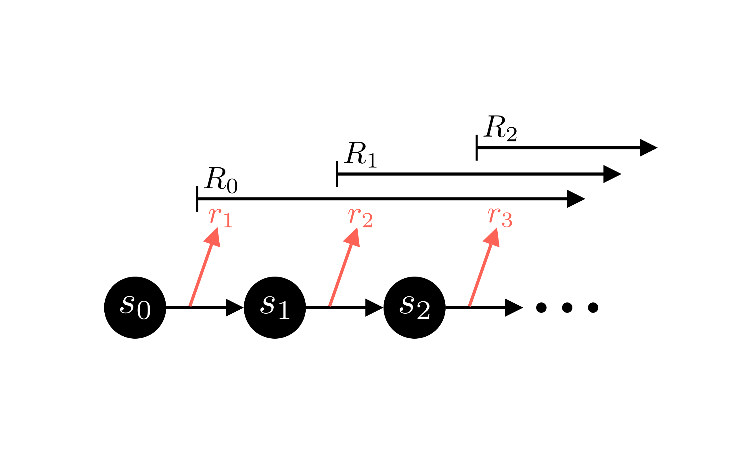
Let’s be as explicit about this as possible.
Remember our trajectory \(\tau = (s_0, a_0, r_1), (s_1,a_1,r_2), (s_2, a_2, r_3),…\). Assume \(T\) time steps \(t\) in a trajectory \(\tau\); \(t \in \left[0,T\right)\), or \(t \in \left[0,T-1\right]\) if you prefer. Now consider the future return \(R^f_t\) at various time steps:
- \(R^f_0\), i.e. \(R^f\) for the first time step (\(t=0\)) in a trajectory, contains all the rewards in that trajectory. Remember the first reward is \(r_1\).
- \(R^f_1\) contains all rewards, except the first reward: \(r_2\) onwards.
- \(R^f_{T-1}\)(the final time step) contains no rewards, because there’s no future!
- \(R^f_{T-2}\) contains only the final reward.
In other words,
\[R^f_{t} = \sum_{t'=t+1}^{T}\gamma^{t'-t-1}r_{t'}\]where T is the total number of time steps in an episode (and we’ve remembered to include the discounting factor \(\gamma\)).
Overwrite your pointers and vocabulary? (Y/n)
With the above argument about not being able to affect the past, it turns out there’s little reason to ever use the original full trajectory return $R$. So take a moment to internalize this concept. From here on out, we’re just going to “overwrite” our previous terminology; any time we say “return” or $R$, we’re talking about this new “future return” or $R^f$. It will be implicit! Let’s modify the policy gradient to use our new understanding of return instead:
\[\hat{g}=\sum_{t=0}^{T}\nabla _{\theta}\log\pi_\theta (a_t\vert s_t)_{\theta _k} R_t\]It looks the same? Oh yes, but now we understand it differently!
Now, how do we actually calculate \(R_t\) for a particular time step? It seems obvious: simply take the discounted sum of all the future rewards! Well, it’s a bit trickier than that, because I don’t have a time machine that goes forward, either.
The obstacle here is that you never have the future rewards for a time step as you’re playing out that step. You only have immediate access to the rewards you don’t care about, those in the past. So you’re forced to keep “rolling out” the trajectory to its conclusion, recording all future time steps, and only then you can accurately calculate \(R_t\) for all time steps.
Yeah ok, but how do you calculate it??
Once you’ve collected the rewards, \(R_t\) is easy enough to calculate in one backward-in-time pass with some simple dynamic programming.
Starting from the final time step, each \(R_t\) equals the reward of the current time step plus the discounted return from the next time step. That is,
\[R_{T} = r_T\] \[R_{T-1} = r_{T-1} + \gamma r_T\] \[\vdots\] \[R_{t} = r_t + \gamma R_{t+1}\]Now just loop this backward in time.
Whew. That seems a lot more tedious than we were hoping for, doesn’t it?

Ok, I’m exaggerating a bit
Now, modern “offline” algorithms aren’t actually this bad. They usually collect short sequences of transitions rather than full trajectories, and store them in a buffer to be sampled and asynchronously learned from. So the “reflection between games” is happening at all times, and the algorithm is “reflecting on all past games,” so to speak, rather than the most recent experience. In other words, in “online” algorithms the state space currently being learned from is the same that’s currently being explored by the active policy. However in “offline” algorithms the current policy (implicit or explicit) sets the explored state space, but the buffer of historical data encapsulates a larger and potentially different state space. There are pros and cons to each approach.
I would like my algorithm to be “online,” meaning I would like to avoid having to collect full episodes before knowing what my return \(R_t\) is. If I could do that, I would be able to learn from the reward of every time step in real time, and update my policy accordingly. The smaller the time lag in learning, the faster I can gain information about my new policy, and update it again. So, how to access the return now instead of later?
The value function
The value function \(V\)’s job is to approximate the return \(R\) at whatever time step \(t\) you need, and to generalize across states. A window into the future!
This is a lot simpler than it may seem. The value function \(V\) answers one question: how good is the state \(s\) to be in? Or, given the state \(s_t\) at time step \(t\), what is the best approximation \(V(s_t)\) of the expected return? With a deep neural network, we can quickly dispatch this question with good old supervised learning.
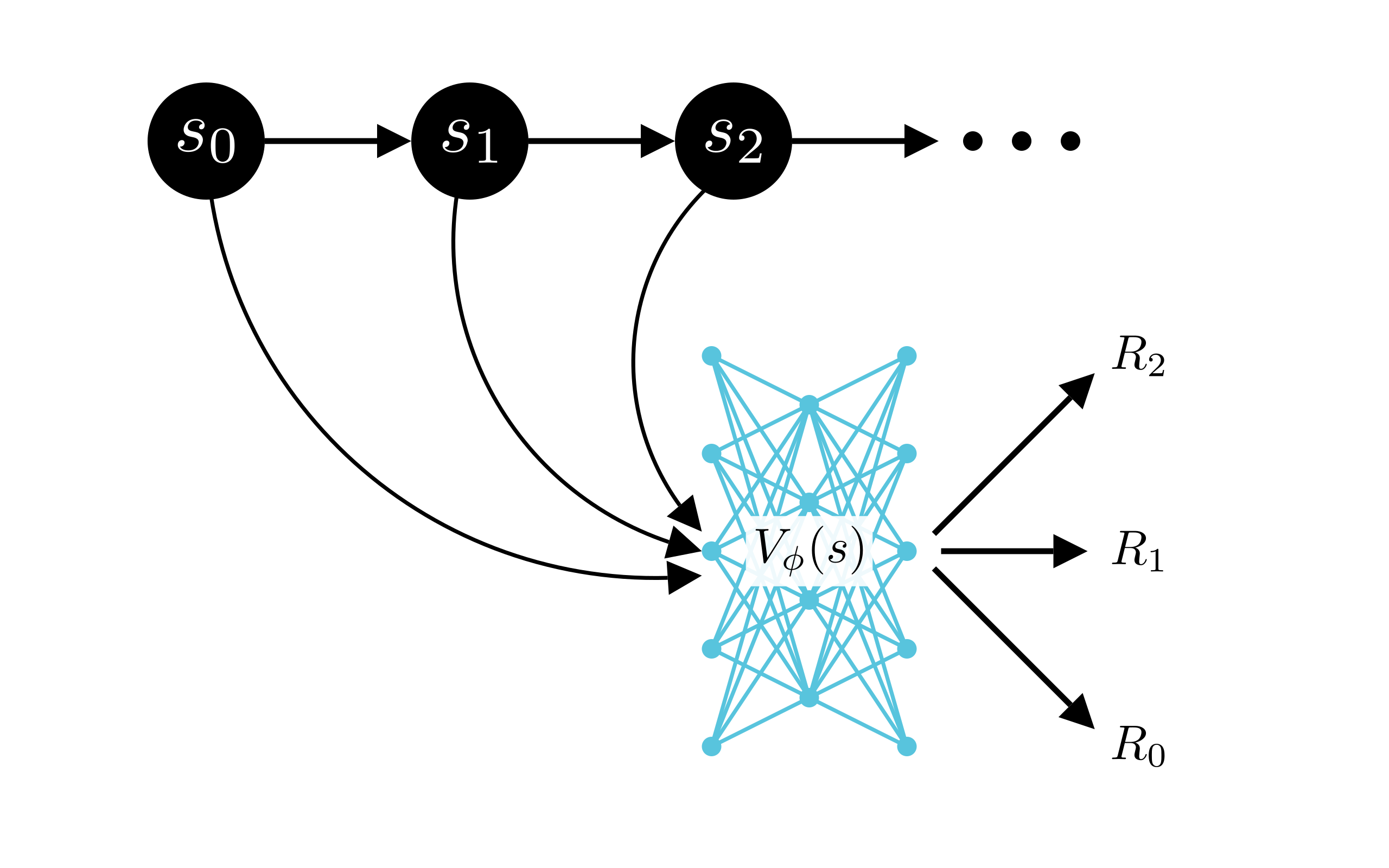
We have a trajectory of states \(s_t\), and at the end of an episode (or the effective time horizon defined by the discounting term \(\gamma\)) we know we’re able to calculate the return \(R_t\) for each time step. We define the loss function for this supervised learning problem as the squared error between the value function \(V\)’s estimate and the actual return:
\[\text{Loss}_{V_t}=\left(V(s_t)-R_t\right)^2\]and minimize this Loss by regression with some kind of gradient descent, training our neural network to predict the return.
And by sticking \(V_t\) in the place of \(R_t\), we almost have the complete policy gradient:
\[\hat{g}=\sum_{t=0}^{T}\nabla _{\theta}\log\pi_\theta (a_t\vert s_t)_{\theta _k} V_t\]Now for a few caveats.
Bias and unstable exploration
This approximation may only see a subset of the state space at any given time, and it may never see the full state space. We cannot assume it is an unbiased estimator unless it has trained uniformly on data from all parts of the state space, and typically that will only be the case once the training is complete, if it happens at all. In parts of the state space which are relatively less explored, it may be very inaccurate, which could lead to learning what the value function says is an optimal policy, but in reality is nonsense.
One of the best solutions to this problem is seen in the popular RL algorithm PPO. Once you’ve understood VPG, you should work your way through TRPO, and then PPO. These links are decent references, though if you feel this blog post helped you understand VPG, let me know in the comments. If there’s enough interest I’ll continue these tutorials!
The gist of PPO
PPO’s goal is to avoid veering too far out into unexplored territory too quickly. It allows the value function time to “acclimate” to its new surroundings and give more accurate estimates, and so the policy is always learning from a “good enough” value function. It accomplishes this by limiting the size of the policy update step by clipping a surrogate loss function - but I won’t digress too much on this point, it requires its own post to do it justice.
Variance
It also turns out that despite removing the noise from past rewards, this simple solution is still quite high-variance in practice. Because of this, it’s difficult for the actor to learn a good policy and to do so quickly. Luckily there are many battle-hardened techniques for reducing variance. Read on for one such technique!
N-step return
What is the lowest bias approximation of the return \(R\) for a state? Well, the return itself! That is, the actual sum of rewards that we calculate.
Hol’ up. Calculating \(R\) requires collecting a full trajectory \(\tau\). Aren’t we trying to avoid that, to learn faster?
Indeed we are. So perhaps we can combine the two approaches. What if I use the actual reward in the next time step, and add it to the value function’s approximation of the discounted return from that point on? Aha, a slightly more accurate estimate! This one step return is shown in the following figure and equation:
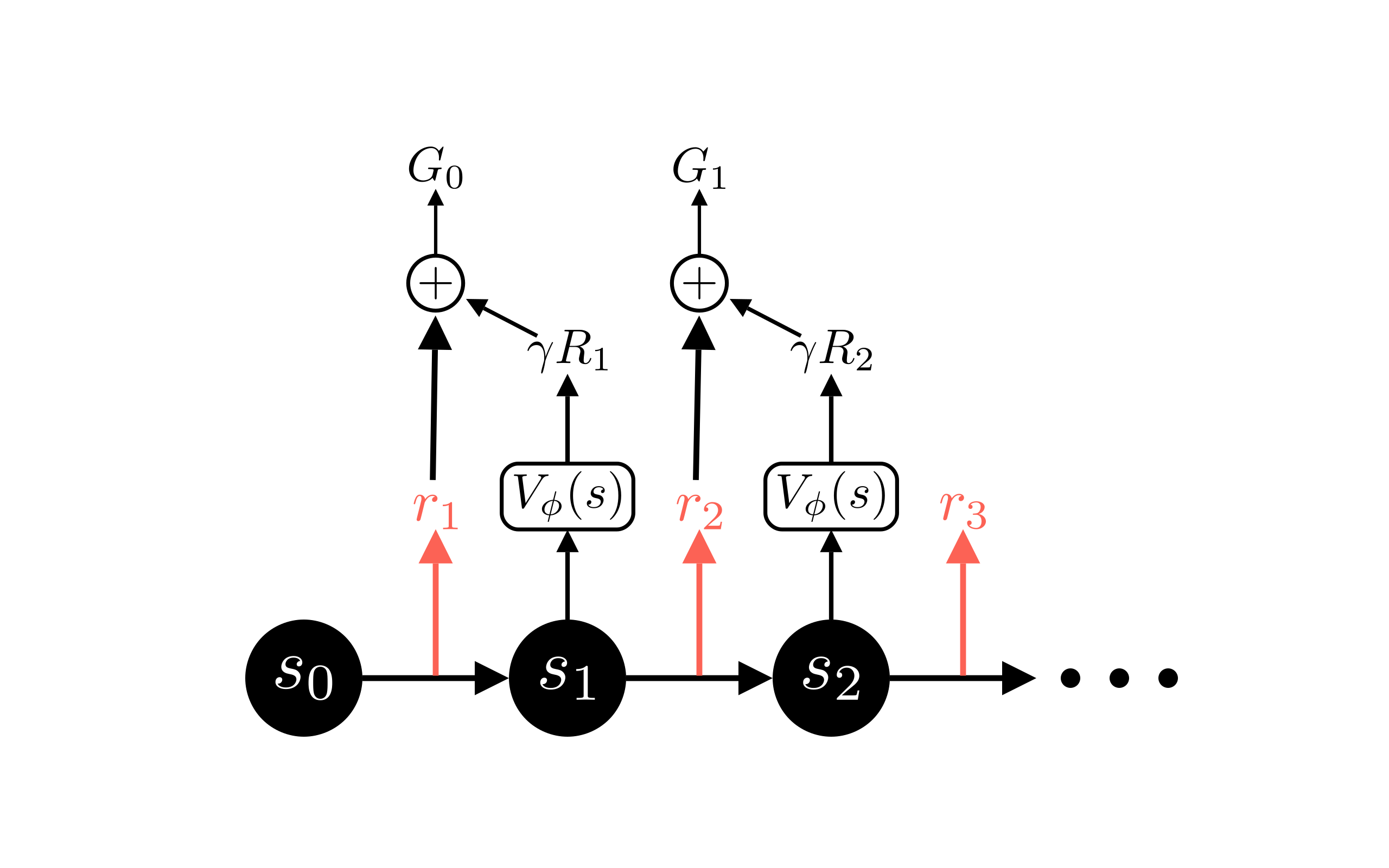
Perhaps we can do better still by using the next two real rewards instead of only one. Or the next three? Each addition will require a slightly longer delay between taking an action and being able to learn from it, because we need to collect a longer sequence out of the full trajectory. This is known as the n-step return \(G\).
\[G_{t:t+2} = r_{t+1} + \gamma r_{t+2}+\gamma^2 V(s_{t+2})\] \[\vdots\] \[G_{t:t+n} = r_{t+1} + \gamma r_{t+2}+ \cdots +\gamma^{n-1}r_{t+n}+\gamma^n V(s_{t+n})\]Now the question becomes: what’s the optimal tradeoff between accuracy and this learning delay? At this point you just need to experiment and see what works best for your problem, but I will tell you this: the answer is somewhere between 100% accuracy and zero delay, as seen in this figure:
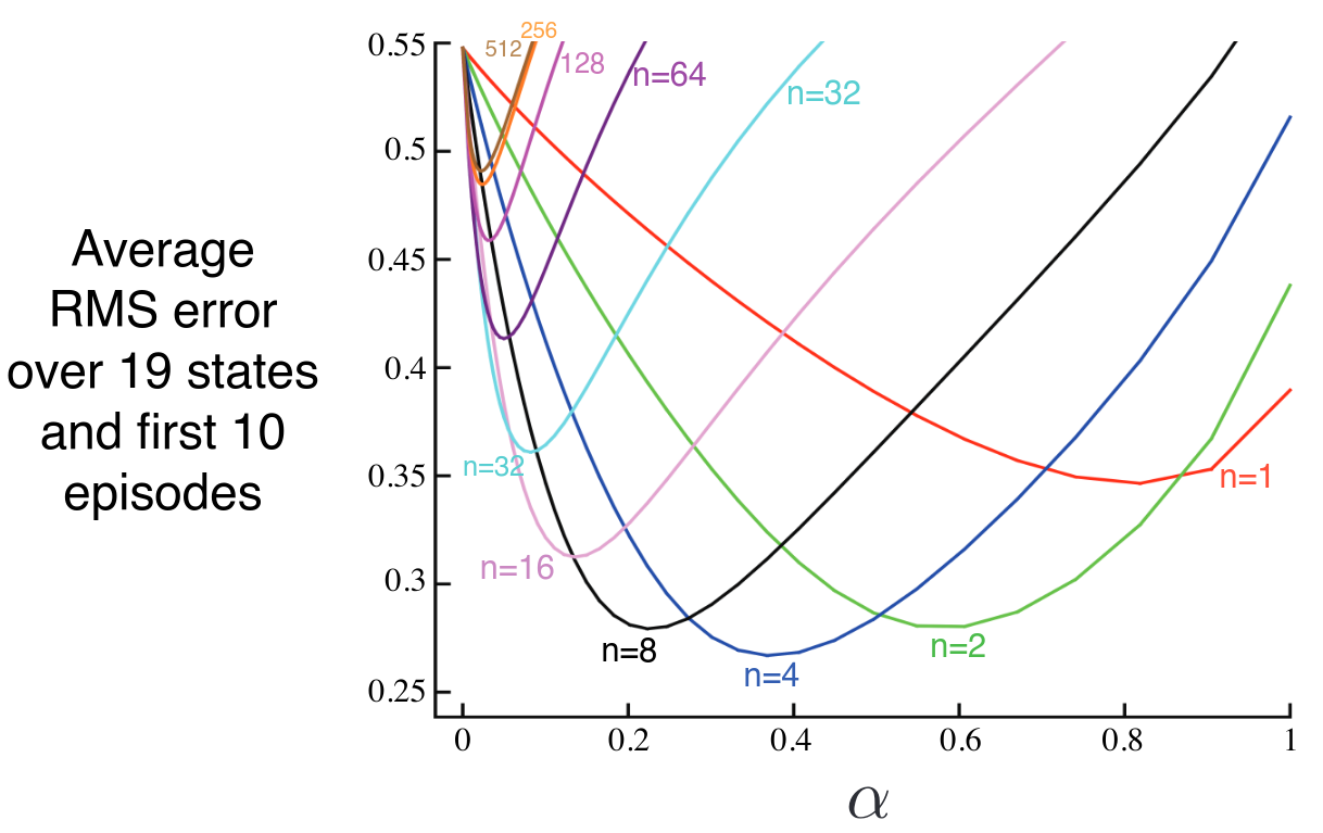
It also turns out you can do even better by doing a weighted average of all of these options: one, two, three, etc. real rewards, followed by an approximation, and also experimenting to see what the right weighting is. There is a similar tradeoff between accuracy and computation speed, yielding a chart like the one above. Optimizing these hyperparameters is problem dependent.
Generalized Advantage Estimation
We have a more accurate approximation with our n-step return \(G\). We’ve left out one important piece, though: advantage. Before we add it, let’s talk about why we need it.
Variance reduction
The n-step return handily deals with the bias problem in approximating the value function, but doesn’t do much to help the variance. To reduce the variance we need to understand where it comes from.
In any trajectory, there are several sources of randomness contributing to what direction it takes as it’s rolled out:
- We may have a random initial state \(s_0\).
- For a given policy \(\pi\) and state \(s_t\), in general we sample actions \(a_t\) from a distribution.
- The environment may have probabilistic transitions. For a given state $s$ and action $a$, in general, the resulting transition to the next state $s_{t+1}$ is also sampled from a probability distribution, \(p(s' \vert s, a)\). We swept this one under the rug until now (and will continue to do so for the rest of this post, so don’t worry).
Each variation at each time step ultimately leads to the variance of the return \(R\). The longer the trajectory, the more pronounced this effect will become. Therefore, we want to remove the effect of this future variation.
Advantage
I’ll start with the punchline: it turns out you can take the expression you want (the n-step return), and subtract another similar expression (a baseline) to reduce the variance of your approximation. Take the following figure as a simple example.
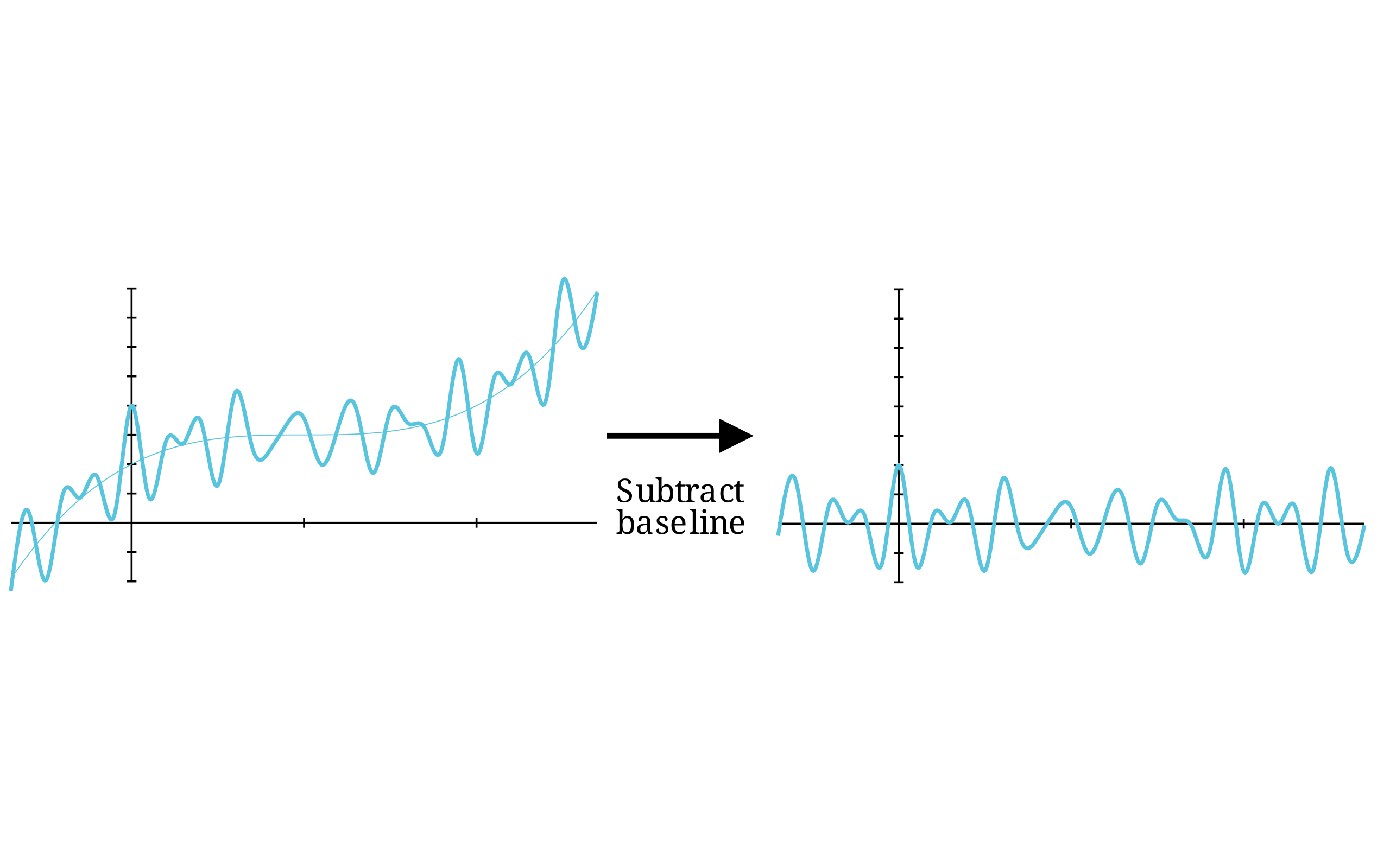
We’re in the business of using “real-time” approximations, so the n_step return is what we’d like a low-variance estimate of. Consider the 1-step return.
\[r_{t+1} + \gamma V(s_{t+1})\]The most common choice for a baseline is the value function, so the above becomes:
\[A_t = r_{t+1} + \gamma V(s_{t+1}) - V(s_t)\]or more generally,
\[A_t = G_{t:t+n} - V(s_t)\]Now hold on. This is just the same as we had before. It’s the n-step return, but for some reason we’re subtracting the value function evaluated on the current state. What’s the point?
Intuitively, the advantage at its most basic level answers the question: how much better is the actual return \(R\) better than my estimate \(V(s)\)? In a sense, it’s a measure of surprise. If taking an action \(a_t\) given the state \(s_t\) and transitioning to a state \(s_{t+1}\) is more rewarding than we think that state is in general (\(V(s)\)), then surely we ought to adjust our policy to do that more often.
With the addition of advantage, we have generalized advantage estimation (GAE) in a nutshell. I’ve focused on intuition here. For more specifics in how these calculations are done, see the paper; your mental picture should now be organized to have all those formalisms swiftly fall into place.
We can now convert our \(V_t\) to \(A_t\).
\[\hat{g}=\sum_{t=0}^{T}\nabla _{\theta}\log\pi_\theta (a_t\vert s_t)_{\theta _k} A_t\]It is worth noting that GAE is not limited to on-policy methods; it can be applied anywhere you use a value function, or even a Q function.
Ok, but why does it actually work?
If the intuition isn’t cutting it for you, see this brief post about why subtracting a baseline reduces variance.
Batched training of neural nets

Finally, we sum the policy gradient over a set \(\mathcal{D}\) of collected trajectories \(\tau\), dividing by the number of trajectories \(\vert \mathcal{D} \vert\) to get the sampled mean of the above equation.
Why? Well, to gain a lower variance estimator of the true policy gradient. This should be quite familiar to you if you’ve ever done mini-batched stochastic gradient descent. Many trajectories averaged together will smooth out the noise from any one trajectory, and better represent the optimal policy gradient.
Policy gradient update
With this, we finally have the full policy gradient!
\[\hat{g}=\frac{1}{\left| \mathcal{D}_k \right|}\sum_{\tau\in \mathcal{D}_k}\sum_{t=0}^{T}\nabla _{\theta}\log\pi_\theta (a_t\vert s_t)_{\theta _k} A_t\]Where \(k\) is the step index in the training loop.
With this term, we can update the parameters of our policy with SGD:
or otherwise use an optimizer like Adam.
Value function update
This is the policy learning taken care of. Now we turn to updating the value function. Recalling its loss function:
\[\text{Loss}_{V_t}=\left(V_\phi(s_t)-\hat{R}_t \right)^2\]We add a sum over all time steps in the trajectory, and a sum over all trajectories in our gathered set of trajectories \(\mathcal{D}\):
\[\frac{1}{\left\vert \mathcal{D}_k \right\vert T}\sum_{\tau\in \mathcal{D}_k}\sum_{t=0}^{T}\left(V_\phi(s_t)-\hat{R}_t \right)^2\]We divide by \(T\) because we’re not doing a sum of log likelihoods like for the policy gradient, but instead are calculating mean squared error.
\[\phi_{k+1}=\arg \min_\phi \frac{1}{\left\vert \mathcal{D}_k \right\vert T}\sum_{\tau\in \mathcal{D}_k}\sum_{t=0}^{T}\left(V_\phi(s_t)-\hat{R}_t \right)^2\]Standing in for the \(\arg \min\), we can use SGD or Adam to compute the update to the value function parameters \(\phi\).
With each gradient descent step, the value function, on average, better approximates the real sum of rewards. The policy then has a more accurate value function with which to adjust its own actions. Together, they explore the state and action space until a locally optimal policy is reached. Though every step is not guaranteed to improve due to approximation error, even this “vanilla” reinforcement learning algorithm can learn to complete simple tasks.
Now you can put all these ingredients together. Convince yourself that you understand the full algorithm!

Go over it and see that everything lines up for you.
Thanks for reading!
Now we can take a look at an implementation in JAX in the next post.