The Reinforcement Learning Problem
Before anything else, define the problem you need to solve.
So, you wanna do RL
This post is the place to start. RL has successfully defeated grandmasters in Go, Dota 2, and is responsible for training ChatGPT. Here we will lay out the reinforcement learning problem, and in future posts I’ll lay out how various algorithms go about solving it.

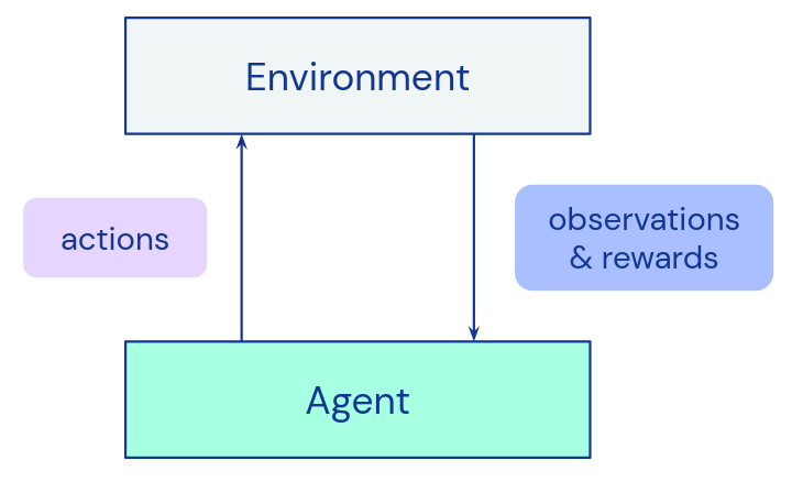
I briefly talk about policies in this post as an example of a solution, with no mention of TD- or Q-learning, which are equally important. For pedagogical/introductory purposes, policies as are slightly more intuitive and straightforward. Don’t let this scare you away from Q-learning, because it is powerful and eminently learnable! Now, without further ado, let’s jump right in. In the standard setup of the reinforcement learning problem, you have an actor and an environment interacting in a loop.

From the environment’s point of view…
The environment is always in a well-defined state \(s\), and given some action received by the actor, it will transition to a new state \(s’\) corresponding to that action. When this transition happens, the environment will spit out a reward \(r\) for transitioning from \(s\) to \(s’\): \(r = R(s,a,s’)\). Eventually some special terminal state is reached. We reached our goal or irrevocably failed the task, and our episode ends. At the beginning of each new episode, the environment can be initialized to an initial state \(s_0\).
This environment is a Markov decision process (MDP): go read about those on page 47 of Sutton and Barto.
From the actor’s point of view…
The actor will take an observation of the environment’s state, process this information, and output an action to the environment. It will then record the reward \(r\) output by the environment, and continue this loop. This reward is the signifier of “good” or “bad” results from the reinforcement learning actor’s actions.
Following this loop forms a trajectory \(\tau\) made up of the states \(s_t\), actions \(a_t\), and rewards \(r_t\) at each time step \(t\). \((s_0, a_0, r_1), (s_1,a_1,r_2), (s_2, a_2, r_3),…\)
“That looks funny,” I hear you say.
The reward time step is offset by one for a few reasons. We don’t get any reward for the first time step \(t=0\), i.e. for initializing the state \(s_0\). Why? We haven’t taken any action yet. Also, the reward \(r\) is associated with both state \(s\) and \(s’\), which live in separate time steps. We have to pick a formalism, so we assign the reward to the latter time step \(t+1\), because the environment returns it at the same time as the next state \(s’\). However, we group it with the former tuple in our trajectory \(\tau\), because it’s associated with the action \(a_t\) we took at that time step \(t\). This tuple organization follows an intuitive loop from the actor’s point of view: “observe, act, get a reward,” then repeat.
“But wait,” I hear you say.
It would make more sense to have a “null” reward \(r_0\) at the beginning which we spit out but don’t do anything with, and form our trajectory like so:
\((r_0, s_0, a_0) (r_1, s_1, a_1),(r_2, s_2, a_2), …\)
The subscripts look nicer, but this doesn’t really end the tuples at natural stopping points.
Often the trajectory is represented without the reward at all, subverting this issue entirely! (Although, this does beg the question of “where do I keep my rewards to learn from?”). Feel free to consider further, but try not to get hung up on this point. Ultimately, we’re representing the same thing, and sometime very soon you will abstract away the whole process. The following example should clear things up.
1D Grid World
A Simple Environment
Let’s consider a 1D grid world, where the goal is simply for the actor to be as near as it can to a particular grid space, and x is the target grid space.
\[\begin{array}{|l||c|c|c|c|c|c|c|} \hline \text{x=4} & & & & & x & & \\ \hline \text{State} &0 & 1 &2&3&4&5&6\\ \hline \end{array}\]Since our goal is to be near to the target space \(x=4\), let’s define a reward function: \(R(s’) = |4-s’| + 4\). Remember \(s’\) is the state we end up in after taking an action.
You dropped this: \(s,a\)
Well well, you’re a quick learner. Yes in general, the reward is a function of \((s,a,s')\). This simple example only depends on \(s'\).
Why \(+ 4\)?
I add the 4 to keep the numbers positive, i.e. a little cleaner, but offsetting the reward function makes no difference to the RL algorithm. I could add or subtract 10,000, and in principle it will still work, especially if you are standardizing the inputs to your neural network.
We see each grid space take on a reward following this function:
\[\begin{array}{|l||c|c|c|c|c|c|c|} \hline \text{x=4} & & & & & x & & \\ \hline \text{State} &0 & 1 &2&3&4&5&6\\ \hline \text{Reward} &0 & 1 &2&3&4&3&2\\ \hline \end{array}\]Now, our actor may start at a random location, but let’s suppose it starts at 0:
\[\begin{array}{|l||c|c|c|c|c|c|c|} \hline \text{x=4} & o & & & & x & & \\ \hline \text{State} &0 & 1 &2&3&4&5&6\\ \hline \text{Reward} &0 & 1 &2&3&4&3&2\\ \hline \end{array}\]where o is the location of our actor. Notice here the initialization of the environment state doesn’t spit out a reward.
Suppose we have 3 actions available to us at a given time step. We can move left, right, or stay put. Encode these actions as -1, 1, and 0 respectively. This environment follows a deterministic state transition, i.e. a left action will always move us left one grid space, and so on. If we bop into a wall, then we stay put.
When we transition to the new state, we obtain the associated reward: \(r = R(s’)\). The goal in the RL problem is defined as maximizing the “return,” or the sum of rewards \(r\) in a trajectory \(\tau\). If you prefer, the trajectory’s return is
\[R(\tau)=\sum_{t=0}^{T}r_t\]Introducing the Policy
The actor maintains a policy \(\pi(a\vert s)\). For a given time step \(t\) in the trajectory \(\tau\), this function outputs the probability distribution of all possible actions \(a_t\), given the state \(s_t\). We can see the optimal policy \(\pi(a\vert s)\) which achieves this goal immediately:
\[\begin{array}{|l||c|c|c|c|c|c|c|} \hline \text{x=4} & & & & & x & & \\ \hline \text{State} &0 & 1 &2&3&4&5&6\\ \hline \text{Reward} &0 & 1 &2&3&4&3&2\\ \hline \text{Policy} &1 & 1 &1&1&0&-1&-1&\text{1, 0, -1 = right, stay, left}\\ \hline \end{array}\]That is, step towards the target, and if you’re on the target, stay put. At the risk of being obvious, let’s show the optimal trajectory following this policy for our actor starting at position 0. Remember a trajectory \(\tau\) follows the form \((s_0, a_0, r_1), (s_1,a_1,r_2), (s_2, a_2, r_3),…\)
\[\begin{array}{|c|c|c|c|c|c|c|l|} \hline o & & & & x & & &s_0=0, a_0=1 &\text{ initial state; no reward}\\ \hline &o & & & x & & &r_1 = 1, s_1=1, a_1=1&\text{ move right}\\ \hline & &o & & x & & &r_2 = 2, s_2=2, a_2=1&\text{ move right}\\ \hline & & &o& x & & &r_3 = 3, s_3=3, a_3=1&\text{ move right}\\ \hline & & & & o & & &r_4 = 4, s_4=4&\text{ terminal state; no action}\\ \hline \end{array}\]At this point the actor receives the final reward and state, and notices it has reached the goal/terminal state. No further actions are taken and the episode ends. Our return, or sum of rewards, is
\[R(\tau)=\sum_{t=0}^{T}r_t = r_1+r_2+r_3+r_4 = 10\]Trajectory? Episode?
For the purposes of this post, the trajectory is just the full episode. In general, a trajectory is any contiguous subsequence of an episode, while an episode is the full sequence from initial state \(s_0\) to terminal state \(s_{T-1}\) for an episode of length \(T\), if it ends at all.
What if: bad grid spaces?
We also could have put “pitfalls” at each end, such that the actor would receive a large negative reward, and the episode could end then, as well. Clearly an optimal policy would involve avoiding these “bad” spaces.
We’ll leave representing and learning the policy \(\pi\), which can be handled by all manner of RL algorithms, to future posts and external resources. This post’s purpose is merely to lay out the problem to be solved.
Let’s make this picture more general so it can describe any environment interaction.
Extending the Simple Picture
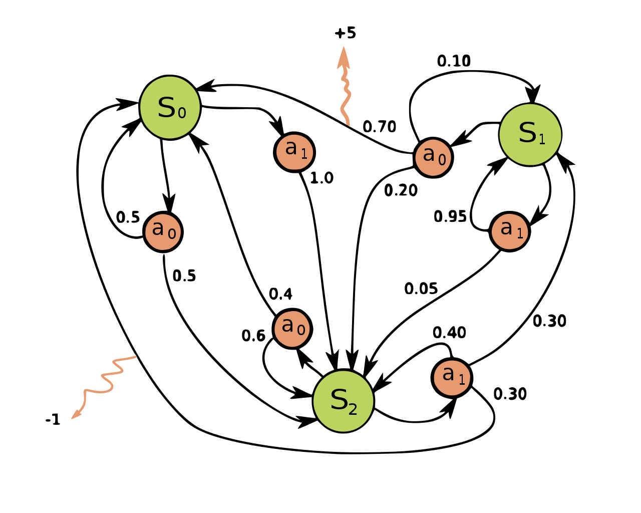
By the way, if this gets to be a bit much, there is a handy picture of an MDP at the bottom. May I suggest opening it in a new tab or window for reference?
Imperfect information
Earlier I said the actor “takes an observation” rather than “records the state.” This is because in general, the observation \(o\) recorded by the actor may be an imperfect representation of the well-defined environment state \(s\).
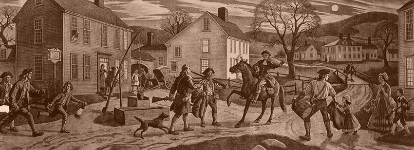
Suppose our actor is Paul Revere, and he is deciding whether to hang one or two lanterns at the Old North Church (action \(a\): 0, 1, or 2, encoding a signal to the militia: “don’t know”, “by land” and “by sea” respectively). There is an advancing British force coming in ships off the coast (state \(s\): 15,000 troops coming by sea).

However, Mr. Revere can only see a boat or two off the coast, and similarly a few carriages shuttling around on land. The British force is concealed by the fog and dark of night
Infinitely long episodes
Next, what if our loop has no foreseeable end? In general this will be the case. Some environments go on forever, and there is nothing in our MDP picture which prevents that from happening.
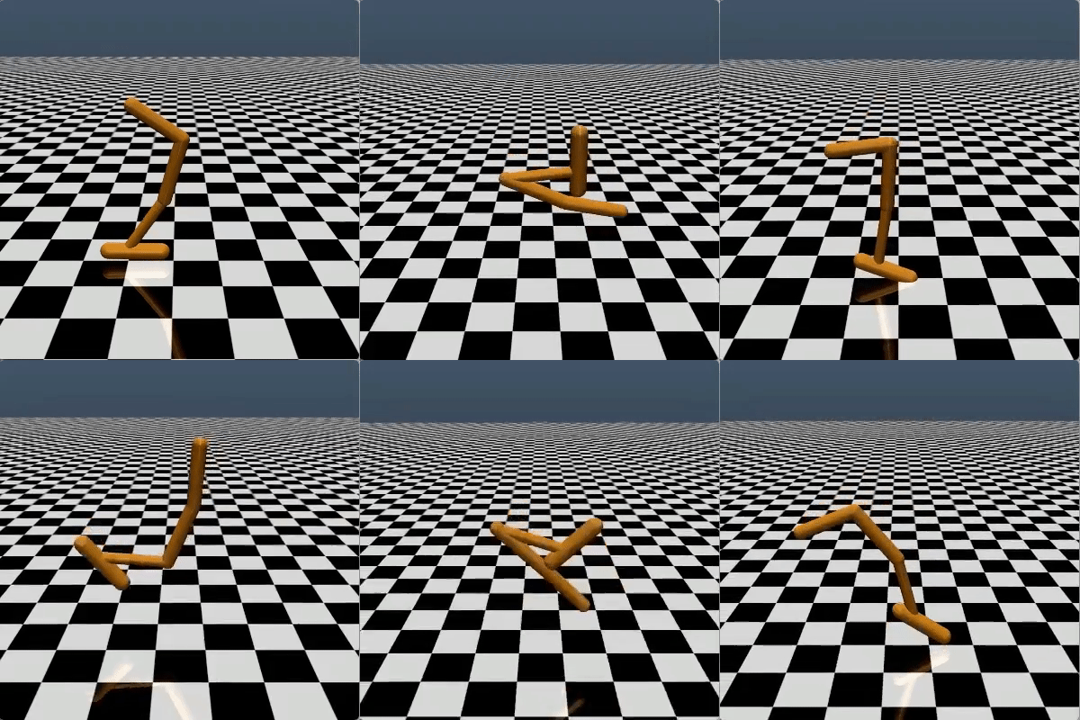
Suppose our actor is a bipedal robot. Its task is to push an AWS server to the top of Mount Everest, because there are excellent ambient temperatures for computing up there. Unfortunately for the robot, every time it gets near the top, its servos freeze over, it loses control of the server rack, and it rolls all the way back to the bottom. And so it will try again until the end of time, or at least the end of its Amazonian overlords. All is well for the robot, who has no shortage of energy or enthusiasm.

How do we support infinite episodes? We simply mandate that every state \(s\) must accept a set of valid actions, and that such actions result in a state transition \((s,s')\). There is nowhere to “end,” and the MDP goes on forever.
Does this picture still support finite episodes? Notice that a state \(s\) can transition to itself \((s’ = s)\). To mark a state as terminal, we only allow it to transition to itself. Technically this is still an infinite MDP: our picture hasn’t changed, it will transition to itself forever. But if we reach a particular state or set of states, we can decide to stop traversing and end the infinite episode prematurely.
Discounted rewards
Now, let me ask you a question. You’ve won a million dollars. Congrats. Would you like your prize now, or in 30 years? Everyone can agree on the answer. If you have it now, you can improve your life, or others lives, now. If you’re worried about self control, stick it in a trust and only touch the dividends. What use is there in waiting?
In other words, reward now is better than reward later, else you’re just wasting time. What’s more, remember our trajectory is infinitely long in general. Ultimately we need to do calculations with the sum to learn from it, and we can’t do that with infinite numbers. To handle this, our actor’s more generalized goal is to maximize the discounted sum of rewards.
\[R(\tau)=\sum_{t=0}^{T}\gamma^tr_t\]\(\gamma\) will usually be set to some number very close to 1, like 0.98. We add the discounting term so that our return converges to some finite value. We can see that as the time step gets further into the future, the discounting factor \(\gamma\) will make reward term decay to 0, and assuming no one reward is infinite, the sum will never be infinity.
We have to go back…
Notice we can recover our original un-discounted picture simply by setting \(\gamma=1\).
Probabilistic state transitions
Our robot from earlier is halfway up the mountain and tries to push forward one more step, but randomly a gust of wind causes him to lose his grip on the AWS server, rolling back down.
What if a particular action \(a\) from a particular observation \(o\) doesn’t always result in the same state transition \((s,s')\)? This is supported by probabilistic state transitions in the MDP. A definite action is taken, then state \(s\) will transition to \(s’\), but \(s’=0\) (the bottom of the mountain) with 5% probability, and \(s’=s+1\) the rest of the time.
In a simulated environment this can be represented by a transition function \(p(s’\vert s, a)\), with a vector of probabilities for all reachable \(s’\) from \(s\), for a particular action \(a\).

That’s our MDP picture and the RL problem; not so bad, is it? Of course, we haven’t done any learning yet! See the next post on VPG for how to learn from interacting with the environment.
My understanding of the subject comes from David Silver’s excellent lectures, Open AI’s spinning up, the 2017 Berkeley Deep RL Bootcamp, Pieter Abbeel’s and Sergey Levine’s various lectures on YouTube, and Sutton and Barto’s “Reinforcement Learning” (which was referenced by the others). These are excellent resources, and I recommend you check them out.