Image Regression Lessons Learned (in JAX)

An exercise in image processing

To get up to speed with image processing, and doing so in JAX, I decided to try something not typically found in your starter image classification notebook. This project was (heavily) modified from the ResNet example found on the haiku GitHub page. Find my code on GitHub.

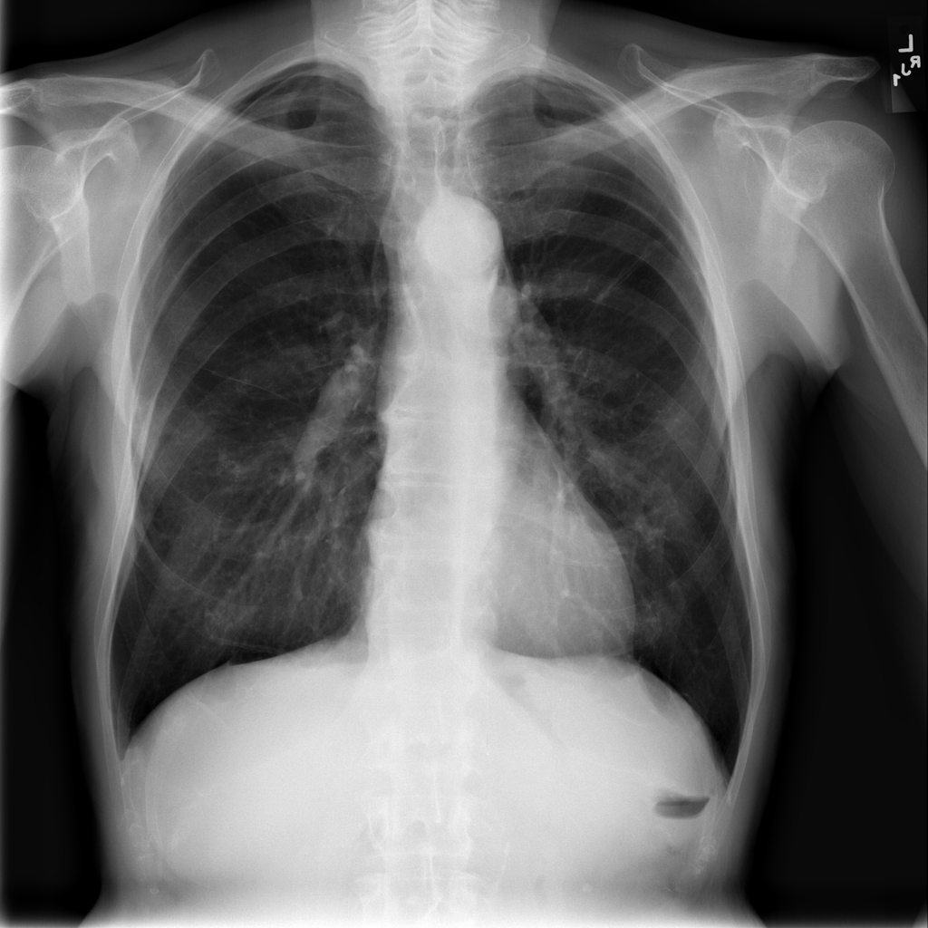
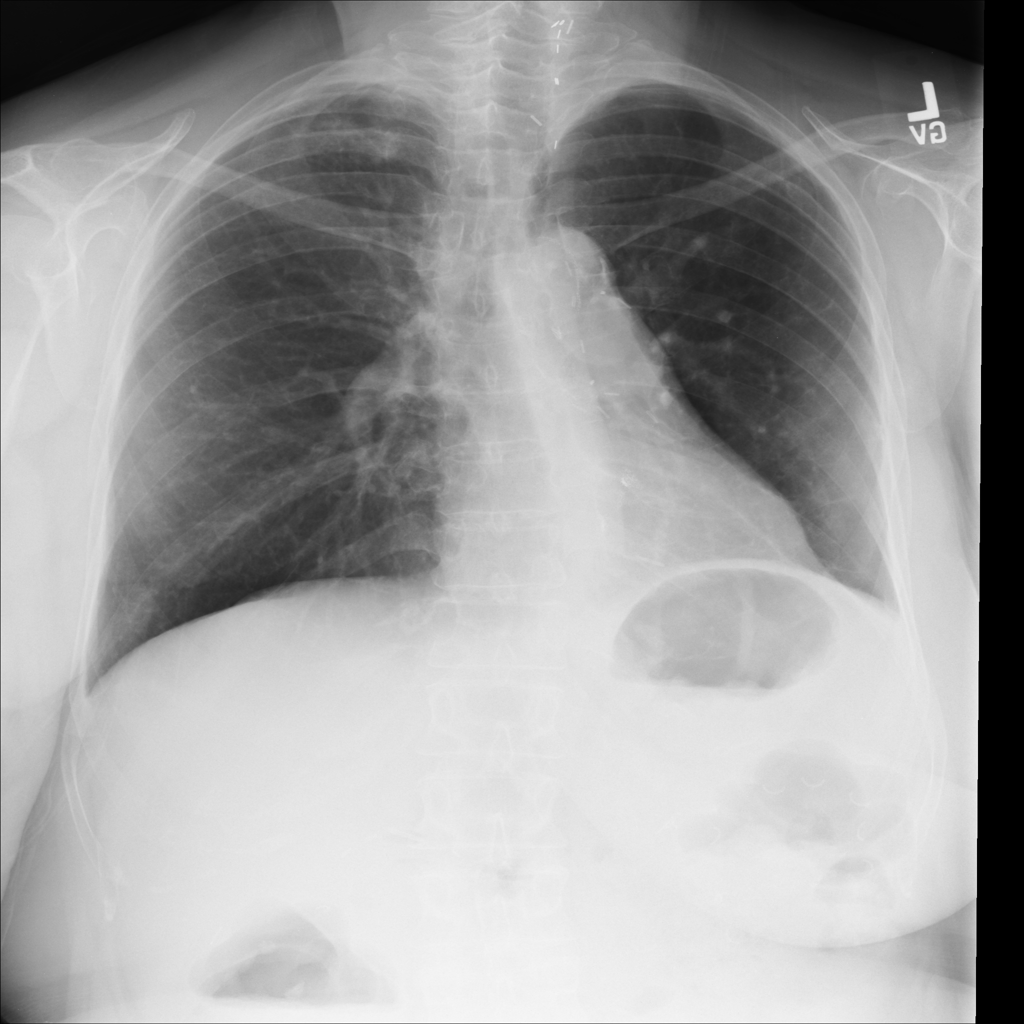
In this post, partly inspired by a list of NN training tips by Andrej Karpathy, I’ll walk through the process of trying to train with low loss on the following dataset.

The problem

~100k samples: x: X-ray images of lungs, y: age label (this is a dataset found on kaggle)
Perform regression from image to age.

Get signs of life, and starter tips

First, you want to make sure your training pipeline actually works and is bug-free. Does your training loss curve reliably decrease and converge to some reasonable (in the context of your dataset) minimum? If it is merely oscillating in place with no sign of training on the dataset, or forever increasing, many things could be going wrong. A bug in your code should always be your first guess. In deep learning, things have a sneaky tendency to fail silently. Without correct code, you could easily spend days chasing barely perceptible gains by tweaking architecture, hyperparameters, trying different optimizers, etc., when it turned out you were computing your loss incorrectly, or simply forgot to apply your gradient.

Start simple

Anything is on the table as far as bugs go, and for this reason it’s important to just get something that works as soon as possible. Start with a relatively low-complexity model, like a basic CNN. If you’re at the point where this seems menacing, just start with a basic MLP, or even linear regression. Start simpler and work your way up in complexity later. Prove to yourself that your training loop is computing loss and gradients and applying them correctly. Prove to yourself that your dataset is actually labelled correctly by going through it manually. Better yet, start from a known working dataset online to prove that your training pipeline works, then swap in the dataset of interest.

Be one with the dataset

Even with correct code, your dataset may have little to no real relationships to be learned at all! For this reason it’s important to attune yourself to the dataset. Really immerse yourself in the relationships you expect and the mechanisms behind them, if any. Any deep learning practitioner needs some data scientist tools in their belt. Visualize, normalize, and clean your dataset.

Once you are satisfied the code is correct, you may still not be training effectively. Your learning rate could be too low, or too high (this is typically the first thing to check). Your model may not have enough capacity to capture the relationships in the data.

Once you’re getting off the ground…

Overfit on purpose

As with any supervised learning problem, your first goal is to overfit the problem. I.e., while paying no mind to the validation loss, see that your model is actually capable of learning the dataset, whether or not it is generalizing well or overfitting. Put another way, make sure you have enough model capacity to accurately map from x to y.

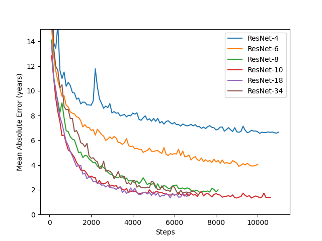
We’ll start with a Resnet with as few layers as we can, and start adding blocks until we get a desirable training error. In this case, let’s consider ourselves satisfied once our training error is less than 1 (estimating age within +/- 1 years). In theory we could go arbitrarily low, effectively memorizing the dataset.

In the figure below, we’ve run each of these Resnet models with early stopping on the train loss. Clearly, increasing the number of blocks (parameters) allows it to more accurately model the dataset, but we see diminishing returns, possibly suggesting that we are nearing the actual relationship that the data actually shows. It’s also possible that not using early stopping and continuing to train these networks would decrease the training loss further. If this weren’t a demo problem, this would be the next thing to check (we’ll skip it in this post for the sake of time).

Here we standardize the inputs to the dataset mean and variance which we’ve calculated separately. We also use Batchnorm for training stability.

Standardize inputs

# ...get the next batch from the dataset... # extract the images images = batch['image'] # Example mean and stddev for an RGB dataset (not used here) # MEAN_RGB = jnp.array([88.94542, 75.03732, 71.47706]) # STDDEV_RGB = jnp.array([71.67816, 66.773605, 65.78593]) stddev_greyscale = jnp.array([42.48881573]) mean_greyscale = jnp.array([126.52482573]) images -= mean_greyscale images /= stddev_greyscale

Overfit — Training loss as we increase model size, for as long as it helps, then a little longer.

Maybe even go a little bigger

It’s often a good idea to leave some wiggle room, rather than using a model that is just barely good enough. It helps to allow the model multiple avenues to approximate the dataset, rather than there being one perfect set of trained weights. As it turns out, having a model that is just barely capable of accurately representing the dataset may actually be detrimental to performance, so it’s best to give it a little extra capacity once you think you’ve hit a minimum. See this paper for thoughts on why this may be the case. Once we start regularizing, a little more capacity won’t hurt either: e.g. because we use only a fraction of the network during training during dropout. We’ll worry about increasing the capacity later if need be. Let’s use ResNet34 from here on.

Regularize

At this point, it’s practically guaranteed we are overfitting the data, particularly as our model size increases. Let’s take a look at the validation error curves from the previous training run.

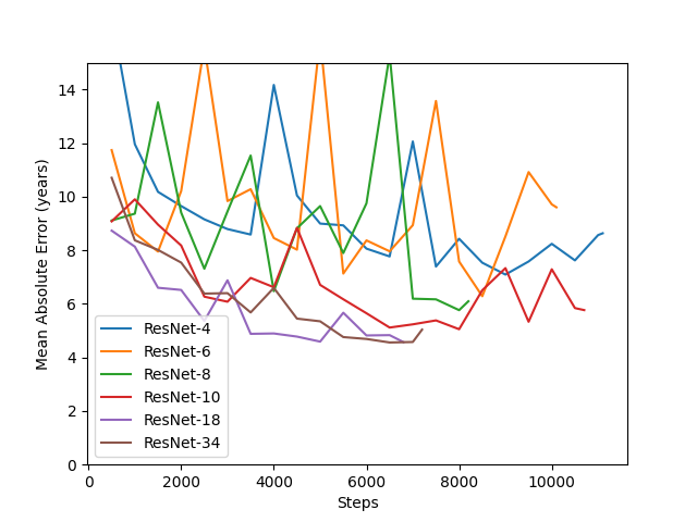
Yes, so we can see that our validation error is quite high.

As a side note, the generalization error is the difference between validation and training errors. If generalization error is higher than training error, (as it is here), this indicates we need to regularize our model. Since this is already the case even at the minimum of the above curves, early stopping will not help us here.

So, our next step is to drive down this validation error with some kind of regularization. This will allow our model to generalize to the dataset’s distribution, rather than overfitting to the training data.

Data augmentation

It’s a kind of regularization.

Often we overfit to particular details in a dataset when, in actuality, more general features are the only ones that apply. Suppose that patients over 60 getting x-rayed are recommended to a particular hospital or clinic for their specialty in older patients. Dependent on the x-ray machine or the post processing of its outputs, perhaps all the x-rays to come out of this clinic have a grey tint, or some form of aberration or postmark around the edges of the image. The neural network will learn (incorrectly, for the global dataset) that grey-tinted x-rays correspond to older patients. Perhaps some similar fluke has patients under 30 have their x-rays mirrored along the y axis.

Enter data augmentation. Images are randomly transformed to be slightly different from the original each time they’re passed through the network, so that incidental details are not learned to be the cause for particular labels. Put another way, we add noise to artificially increase the size of the dataset. (If getting more data is a relatively cheap option, you should absolutely do that first).

RandAugment is the name of the game at the time of this writing, appearing to have the best performance out of comprehensive image augmentation techniques. It blends many different kinds of classic image augmentations, from contrast to translation.

However, dependent on the type of image to be classified or regressed, don’t blindly use augmentations that would obscure necessary info to you. Use common sense here.

Here’s the preprocessing code implementing RandAugment

# Each of these layers is implemented as a function in JAX # in the same file, preprocessing.py randomLayers = [ flipX, translate, color_degen, auto_contrast, equalize, random_contrast, brightness, cutout, rotate, ] def randomAugmentJax(images, rng, policy, augmentations_per_image = 3, rate = 10/11): # For each image, we're going to want a different rng, so we need to split keys = jax.random.split(rng, images.shape[0]) def apply_rand_layer(image, layer_select_key, layer_key): randIndex = jax.random.randint(layer_select_key, (), 0, len(randomLayers)-1) for i in range(len(randomLayers)): image = jnp.where(randIndex == i, randomLayers[i](image, layer_key, policy), image) return image # Now, we need to define a function we'll vmap to our images def augment(image, loop_key): #within this function, we just copy the rand_augment apply original_image = image for _ in range(augmentations_per_image): # get a skip uniform random number loop_key, skip_key, layer_select_key, layer_key = jax.random.split(loop_key,4) skip_augment = jax.random.uniform(skip_key) #skip based on rng above (identity) #else, apply a random layer to the input image = jnp.where(skip_augment > rate, original_image, apply_rand_layer(image, layer_select_key, layer_key)) return image return jax.vmap(augment)(images, keys)

With data augmentation — Training and validation loss upon adding data augmentation.

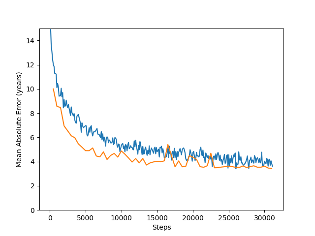
The clear difference here is our validation loss tracks the training loss curve. It isn’t a one-to-one comparison, as data augmentations aren’t applied during eval, so we expect the training loss to be artificially higher. However, as the training loss decreases, the validation loss does as well; they don’t split apart early on as before, with an increasing generalization error. This gives us confidence that we can continue training for a long time without overfitting. We see our validation loss drops from 4.4 to 3.4. Now we’re seeing some results!

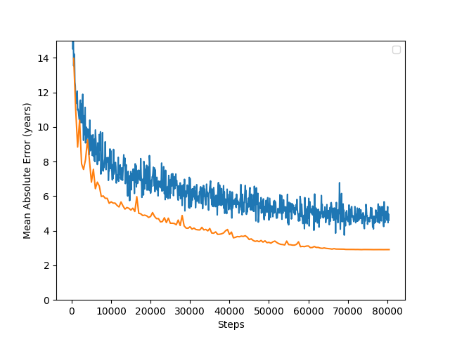
I used early stopping here, but it is likely the validation loss would decrease even further. Additionally, a run I did before writing this post with the same parameters, only adding dropout to the final MLP after the ResNet blocks, got down to 2.91 years mean absolute error when taken to 80k training steps. (Dropout rate was set to 0.25). With that in mind, let’s turn on dropout for the rest of this post.

With dropout — Training and validation loss upon adding dropout.

Speed is the key

While doing all these tasks, your concern should also be speed of training for a low iteration time.

I recommend you don’t use the python multiprocessing library for data augmentation: inter-process communication is too slow because it writes to disk, and you’ll be moving a lot of data around. There are python libraries out there which purport to use RAM for communication, but I did not find them to be particularly plug-and-play.
Instead, learn to use tfds for your data pipeline and dataset creation via their examples and documentation. It may seem like a big hurdle at first, but it will pay off in speed, and it’s applicable to any supervised learning problem you can imagine. (If you’re using pytorch, there is a similar dataloader for you to learn).

Here’s the tfds code preparing the dataset pipeline including some preprocessing

import tensorflow_datasets as tfds def load_dataset(split): # Maximize batch size for the available VRAM # Bigger images & bigger networks = smaller batch size imgSize = imgSizes[FLAGS.img_size_num] resNetRelSize = resnetSizes[FLAGS.resnet_num] / 50 batchSize = nearest2(int(FLAGS.batch_size/resNetRelSize*(128/imgSize)**2)) train_dataset = tfds.load(datasetName, split=split) num_datapoints = train_dataset.cardinality().numpy() train_dataset = train_dataset.repeat().shuffle(1024) train_dataset = train_dataset.map(lambda x: (preprocess(x, True)), num_parallel_calls=-1) train_dataset = train_dataset.batch(batchSize).batch(jax.local_device_count()).prefetch(-1) train_dataset = tfds.as_numpy(train_dataset) return train_dataset, num_datapoints # Found in preprocessing.py def preprocess(x): # This is a little barebones; before moving preprocessing to GPU, # everything was done here via tfds on cpu. x,y = deconstruct(x) if x.get_shape()[2] == 1: x = rgb(x) # convert greyscale to 3 channels for uniform architecture. x = cast_fn(x) return reconstruct(x, y)

This said, if you’re doing all your data preprocessing (e.g. image augmentation) in tfds, you might find you’re CPU-bottlenecked; this was the case for me. With access to highly optimized libraries which can easily execute batched operations on the GPU, or better yet, multiple GPUs (JAX!), you would be remiss to ignore that possibility for your data augmentation. GPUs are not just for neural networks! When in doubt, see if you can implement your preprocessing as part of your network, with a flag for training/eval. This enabled me to go from 20 to near-100% utilization across 3 GPUs.

This code defines the network, but importantly includes preprocessing steps on the GPU in JAX!

def _forward( batch, is_training: bool, apply_rng=None ) -> jax.Array: """Forward application of the resnet.""" images = batch['image'] # Do preprocessing on the GPU!! # randomAugmentJax is found in preprocessing.py if is_training: apply_rng, aug_rng = jax.random.split(apply_rng) images = randomAugmentJax(images,aug_rng,get_policy(), thruLayer=FLAGS.thruLayer, onlyLayer=FLAGS.onlyLayer) # Normalize the inputs on the GPU!! STDDEV_RGB = jnp.array([42.48881573]) MEAN_RGB = jnp.array([126.52482573]) images -= MEAN_RGB images /= STDDEV_RGB net = resnets[FLAGS.resnet_num](FLAGS.layer_size, resnet_v2=FLAGS.model_resnet_v2, bn_config={'decay_rate': FLAGS.model_bn_decay}) mlp = hk.nets.MLP( output_sizes=[FLAGS.layer_size, FLAGS.layer_size], activate_final=True ) yHold = net(images, is_training=is_training) y = hk.BatchNorm(True, True, FLAGS.model_bn_decay)(yHold, is_training=is_training) y = mlp(y, FLAGS.dropout_rate, apply_rng) if apply_rng is not None else mlp(y) # skip connection y = y + yHold y = hk.Linear(1)(y) # No final activation return y.flatten() # Transform our forwards function into a pair of pure functions. # This will later be run on all devices with jax.pmap() forward = hk.transform_with_state(_forward)

It may also be worth using half precision (f16) computation. I won’t get into it here, but the code found on the accompanying GitHub (link at the bottom of this post) allows this by simply changing the mp_policy flag to 'p=f32,c=f16,o=f32'. In my testing this approximately doubles the speed, sometimes at the cost of training stability (you are likely to see NaNs until you fiddle with your learning rate and batch size to make them go away). So far I haven’t found much difference in the overall performance.

Last but not least, balance workload between CPU and GPU so that you’re not bottlenecked anywhere. This may be more hassle than it’s worth, but is worth considering if you have nothing to do but wait for your training runs to complete.

Further optimization

Hyperparameter tuning

Once you have a reasonable h-param range and decent performance, optuna is your friend, but not before. You may have bugs in your code, or the model may under/overfit without the right details as above.

One of these hyperparameters may even be deeper networks. Now that we’ve added augmentation, we may squeeze a few % more out of the data with a higher capacity model.

I will leave this as an exercise for the reader :) .

Modern architectures and more

I did not touch on it in this post, but at this point if the application requires, it may be worth checking out newer networks. Checking out the ImageNet leaderboard shows Vision Transformers, among many others, outperforming ResNet. However, you may find these have their own trade-offs, perhaps requiring much larger datasets or pre-training to get this performance.

Furthermore, in my experience, feature extraction from / fine-tuning a pre-trained network (e.g., a ResNet-50 trained on ImageNet) is likely to give you astounding results with minimal training time, in particular if your dataset of interest is similar to the images found in the larger dataset the network was pre-trained on. ImageNet may not help much with X-rays, but other applicable pre-trained networks may be out there.

Good luck in your exploration!

Thanks for reading! Find the code on GitHub.