CoachRL Back End
Digging in to dirty details
See previous posts for discussion of habits and rewards, and the daily use of CoachRL. This post covers the technical details which power the project. See the GitHub Repo.
Outline
Someday, this may become neatly contained in an iPhone app. For now, it is composed of several programs stitched together. First I’ll lay out these components, and touch on RL frameworks. I’ll talk about data pipelines, then I’ll cover the usage of the trained model to output daily suggestions. Finally, we train the model in simulation before introducing it to the real world.
Ingredients
- A Mac/Linux device. (Underlying libraries used do not currently run on Windows, though this could be changed).
- A device on which you can install the messaging app Telegram; used for notifications and requesting rewards for completing tasks.
Optional but recommended:
- A tablet, for a daily to-do list without rewriting your routine every day. I use an iPad with GoodNotes.
- An iPhone for auto-weight tracking.
Software used:
- A Renpho Bluetooth scale for weigh-in, with the associated iPhone app.
- iCloud to transfer weight data to a local csv file.
- Google sheets for an interactive log of daily habits, and running averages.
- Python, and many libraries, most importantly Acme from Deepmind, which uses a JAX implementation of PPO. In the future I plan on switching to MPO/MuZero for sample efficiency and performance. Also, libraries for communicating with iCloud and Google sheets. CoachRL shoots daily statistics and provides rewards via a Telegram interface, handled in Python with their bot API. (Any questions on this point: please leave a comment below).

RL Frameworks
This project originated in PyTorch, using Stable Baselines 3. However, scaling actors used a lot of overhead, killing the benefit of parallelizing. Furthermore, extending SB3 was not very intuitive, which limited its usefulness for more advanced use-cases. I cast about for good libraries for parallelization in RL, and RLLib seemed to be a popular choice.
Before settling on this, I read Google is shifting to JAX from Tensorflow for its internal deep learning use cases. If we assume Tensorflow to be the industry standard for production deep learning, and its creators have come up with something more performant, then I’m not going to argue.

(n.b. JAX is using TPU and NumPy is using CPU in order to highlight that JAX's speed ceiling...)."
A recent paper out of Berkeley additionally saw a 16x speedup using JAX over PyTorch, enabling fast (20 minutes!) in-the-wild robot locomotion learning - something previously thought to be impossible due to sample efficiency. Read more about why JAX rules here. I found Acme, geared towards JAX, while using Tensorflow, to be the most comprehensive, maintained, and extendable framework.
Data Pipelines
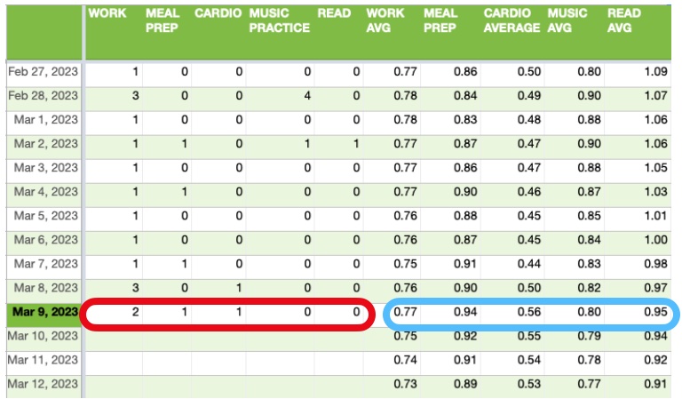
What data are we processing, and what observation does the RL algorithm receive? Every day, you perform your habits to a certain level. For example, perhaps I go for a 30-minute run and practice violin for 15 minutes. I would manually input these values into the Google spreadsheet.
The spreadsheet maintains a daily record of the exponential moving average (EMA) of the habit performance, normalized to your goal (see below figure in blue). Suppose my goal is to run 30 minutes a day, 5 days a week. If I don’t run at all, I would input a 0, and if this goes on for long, the EMA would eventually go to 0 as well. If I ran today for 30 minutes, I would input a 1, which would be normalized to 1*7(days in a week)/5 (days to run per week). 7/5 would be used as today’s update to the ongoing EMA, which will eventually converge to 1 if interspersed with two 0’s per week. The exact values and normalizations can be changed to suit your needs. Inputting 30 for a 30 minute run would work, so long as you’re normalizing it to 1 in the EMA calculation. (1 is assumed to be the optimal value for all goals). This is repeated for every daily habit.

Now, if that sounds tedious, I agree! Having to manually input your habits every day, planning exactly what to do to meet your goals, etc. is a right pain. What if we could manage our habits without having to manually input anything? That is one problem we are here to solve.
Other Data Collection
If one’s goal is to “be healthy,” one may more concretely define this as maintaining a certain weight, body fat percentage, resting heart rate, or all manner of health-related data. While this section can apply to any manner of metrics (perhaps not even health-related), I’m going to stick with weight.
Now, you’re going to have to actually weigh yourself and punch that in to the spreadsheet. No getting around it. Since our goal is to avoid tedium and pain, let’s be slightly smarter about this. I step on a scale every day, which connects via Bluetooth to my iPhone. An automation app on the phone saves this health data once a day to iCloud, which CoachRL can then access and stick in the spreadsheet for you. All that is required of me is grabbing my phone and stepping on the scale. The enterprising user can consider other ways to automatically collect data that is important to them.
How to avoid manual habit entry?
Get a reinforcement learning algorithm to do it for us. All the pieces required to do this have been explained. Now, let’s put them together.
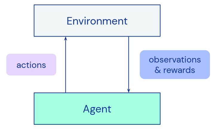
As you may recall, a reinforcement learning algorithm progresses through a trajectory of time steps. Each time step is composed of an observation, an action, an observation following that action, and a reward associated with the transition. Read Sutton and Barto for more details.

The observation is a vector of yesterday’s EMAs: one entry for each habit. Depending on the EMA, we will want to take a different action. What if we are falling behind on our running schedule?
The action taken by the actor is today’s planned level of performance for every tracked habit, based on yesterday’s EMA. If we’re behind our running schedule, run today!
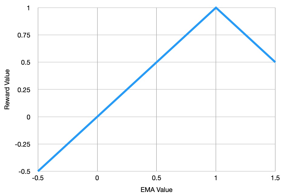
The reward is simply 1-mean(abs(1-observation)): see below figure. If all the EMA values yesterday are at 1 (perfectly aligned with the goals of all habits), then the reward is 1. Any deviation will cause the reward to linearly decrease from this max value. We add 1 to make rewards (usually) lie between 0 and 1, just to keep it intuitive.

Beyond technical details, this is it! The RL actor performs inference on new observations, probabilistically selects actions for each habit, which is then filled in to the Google spreadsheet via the Google Docs API in Python.
Now, if your actions for any reason disagree with what the RL actor spits out, simply edit those values in the spreadsheet. If they consistently deviate, a little massaging of the output before it is filled into the spreadsheet is in order. For instance, if you are “coached” to run, work out, stretch, and play basketball in the same day, you may think this is not realistic for your schedule. In this particular case, I (in Python) randomly select one of those marked active, and set the rest to 0. Any massaging is also implemented when training the model.
Model and Environment Setup
Most of my time was spent creating an environment, grokking iCloud and Google Sheets APIs, and tweaking how actions were processed as I learned about the algorithm’s behavior. A simple N-day rolling average of habit performance was replaced by an exponential moving average halfway through the project. This hugely improved previous erratic behavior: instead of a number dropping out of the dataset entirely once per day, the EMA smoothed this effect out over time.
I did not have a good intuition for how large a network may be required, how many samples, what hyper parameters, etc., were necessary for optimal performance. More often than not, when I tackled strange behavior in the training with creative feature engineering, it ended in more confusion and was ultimately retconned in favor of splitting into multiple actors for the huge action space (10^15 possible combinations for 23 habits with varying action space sizes), one actor for every 5 habits or so.
Finally, the PPO implementation in Acme did not support MultiDiscrete action spaces. That is, 3 possible actions for habit A, 5 possible actions for habit B, and so on. To fix this, given neural network. Taking inspiration from the Stable Baselines codebase, I wrote a similar implementation in JAX, a sample of which is below. See the GitHub Repo.
Simulation Training
Before thinking about training in simulation, I made an environment for reading EMAs from Google sheets, inputting this observation into the model, massaging the output a little, and writing the result back into Google sheets. All that was needed to simulate this process was to replace the calls to the Google Docs API with reading and writing from a queue whose elements represented all actions and EMAs for the day, and calculating said EMAs in Python instead.
Future work
Why bother with the RL model? Well, you may not know the optimal arrangement of your habits every day, or you might not want to slog through manually crafting hard-coded rules. Furthermore, perhaps there are long-term correlations between habits. Perhaps exercise gives you more energy long-term, causing you to get your work done in less time, leaving room for other habits. In the long run, training the model on real life data from the individual will give the best results. This was the main motivation for using RL in the first place.
However, sample efficiency prevents PPO from accomplishing these tasks. 1-5 million samples may be alright in a simulator with multiple actors in parallel, but most people don’t have time to wait that many days to get a good recommendation. This value may be lower when fine tuning a model from simulation on real life data, but is still substantially too large.
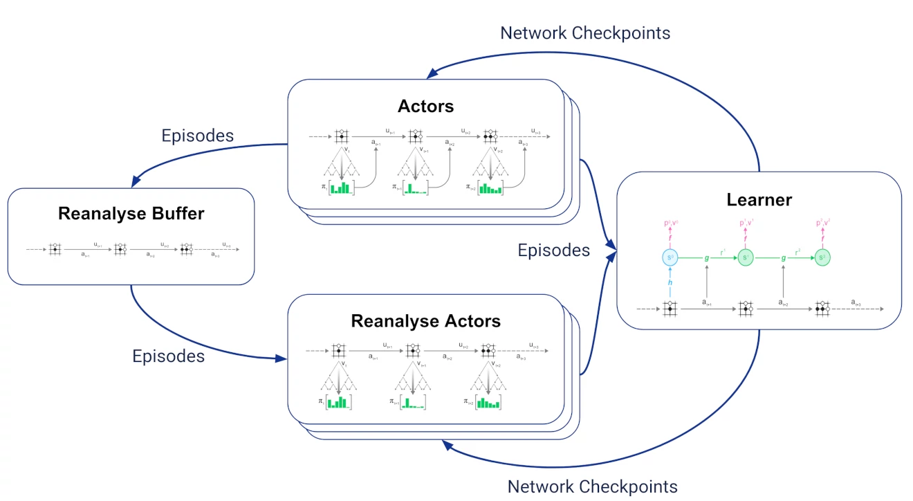
The solution is to use a more sample efficient algorithm. For various projects with costly actions (in particular, PRL), I reviewed the literature in late 2022 and experimented with different RL algorithms to gain optimal sample efficiency. The two that rose to the top in this regard were MPO and MuZero (and follow-up papers). MuZero in particular has stellar performance in the discrete domain, because of its usage of Monte Carlo Tree Search, and stellar sample efficiency largely because it is able to “Reanalyse” the data.

EfficientZero takes this sample efficiency further. (See my implementation and explanation of EfficientZero in blog posts to come!) As one can imagine, this comes at the cost of computational efficiency. However, since the time between steps for our environment is a full day, this is not a dealbreaker for us. While I have moved on to other projects in the meantime, I plan on updating this to use one of these more sample-efficient algorithms to take advantage of this long term “cross pollination” of habit effects. I hope this will result in a more holistic recommendation policy.

Finally, something I found necessary to gain optimal performance for every habit recommendation was to split habits into groups of 5 or so. My use case consists of 23 habits, each with multiple possible actions (up to 20). This is an extremely large action space! This splitting is less than ideal, because it requires more manual work, but particularly because you lose some of the possibility of getting aforementioned “cross-pollination.” It is possible I did not have the patience/compute power to make give optimal recommendations with a single network, or perhaps I simply wasn’t using a large enough network for the task. More reading and experimenting required.
Thank you for reading; suggestions are welcome in the comments below! This article was already pretty long, so I skipped over many details; please feel free to ask! See the GitHub Repo.
See this short post for other Acme issues I resolved surrounding multiple GPUs and parallelization.